
Self-Balancing Robot
This article describes the design of a simple Self-Balancing Robot. It all started as a funny student self-project and then evolved as new teaching platform in the 2nd year control class as it requires State-Space understanding. You'll find here about everything you may need to grab the control fundamentals, build and program your own robot if you wish. All the parts are easy to find or to prototype using home CNC or 3D printing.
The robot in action, after developing an Android control app:
1. Non-Linear Mechanical System
1.1. Modeling
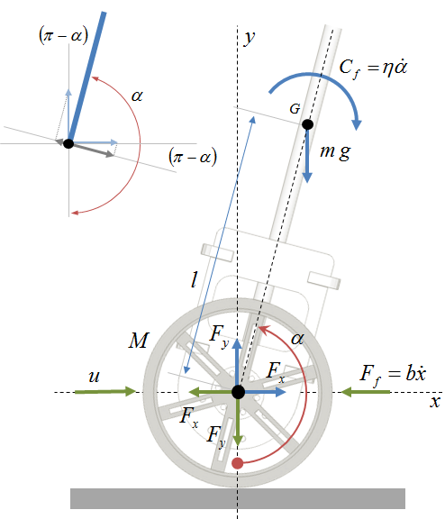
Summing Forces on the Pendulum @G
$m\ddot{x}_G=F_x$ | [1] |
$m\ddot{y}_G=F_y-mg$ | [2] |
Summing Moments on the Pendulum @G
$\displaystyle{J}\ddot{{\alpha}}={l}{\left({F}_{{{x}}} \cos{{\left(\pi-\alpha\right)}}-{F}_{{{y}}} \sin{{\left(\pi-\alpha\right)}}\right)}-\eta\dot{{\alpha}}$ | |
$\displaystyle{J}\ddot{{\alpha}}=-{F}_{{{y}}}{l} \sin{{\left(\alpha\right)}}-{F}_{{{x}}}{l} \cos{{\left(\alpha\right)}}-\eta\dot{{\alpha}}$ | [3] |
Summing Forces on Cart @{0,0}
$\displaystyle{M}\ddot{{{x}}}+{b}\dot{{{x}}}+{F}_{{{x}}}={u}$ | [4] |
Shift forces from $\displaystyle{\left\lbrace{x}_{{{G}}},{y}_{{{G}}}\right\rbrace}$ to $\displaystyle{\left\lbrace{x},{y}\right\rbrace}$
$\displaystyle{x}_{{{G}}}={x}+{l} \sin{{\left(\alpha\right)}}$ | $\displaystyle\dot{{{x}}}_{{{G}}}=\dot{{{x}}}+{l}\dot{{\alpha}} \cos{{\left(\alpha\right)}}$ | $\displaystyle\ddot{{{x}}}_{{{G}}}=\ddot{{{x}}}+{l}\ddot{{\alpha}} \cos{{\left(\alpha\right)}}-{l}\dot{{\alpha}}^{2} \sin{{\left(\alpha\right)}}$ |
$\displaystyle{y}_{{{G}}}=-{l} \cos{{\left(\alpha\right)}}$ | $\displaystyle\dot{{{y}}}_{{{G}}}={l}\dot{{\alpha}} \sin{{\left(\alpha\right)}}$ | $\displaystyle\ddot{{{y}}}_{{{G}}}={l}\ddot{{\alpha}} \sin{{\left(\alpha\right)}}+{l}\dot{{\alpha}}^{2} \cos{{\left(\alpha\right)}}$ |
| [1] → | $\displaystyle{F}_{{{x}}}={m}\ddot{{{x}}}+{m}{l}\ddot{{\alpha}} \cos{{\left(\alpha\right)}}-{m}{l}\dot{{\alpha}}^{2} \sin{{\left(\alpha\right)}}$ | [5] |
| [2] → | $\displaystyle{F}_{{{y}}}={m}{g}+{m}{l}\ddot{{\alpha}} \sin{{\left(\alpha\right)}}-{m}{l}\dot{{\alpha}}^{2} \cos{{\left(\alpha\right)}}$ | [6] |
First governing equation
| [4], [5] → | $\displaystyle{\left({M}+{m}\right)}\ddot{{{x}}}+{b}\dot{{{x}}}+{m}{l}\ddot{{\alpha}} \cos{{\left(\alpha\right)}}-{m}{l}\dot{{\alpha}}^{2} \sin{{\left(\alpha\right)}}={u}$ | [7] |
Second governing equation
| [3], [5], [6] → | $\displaystyle{\left({J}+{m}{l}^{2}\right)}\ddot{{\alpha}}+\eta\dot{{\alpha}}+{m}{g}{l} \sin{{\left(\alpha\right)}}+{m}\ddot{{{x}{l}}} \cos{{\left(\alpha\right)}}={0}$ | [8] |
Solving [7] and [8] gives:
$\displaystyle\ddot{{{x}}}=\frac{{{b}{l}^{2}{m}\dot{{{x}}}+{J}{b}\dot{{{x}}}-{l}^{2}mu-{J}{u}- \cos{{\left(\alpha\right)}}\dot{{\alpha\eta}}{l}{m}-{J} \sin{{\left(\alpha\right)}}\dot{{\alpha}}^{2}{l}{m}- \cos{{\left(\alpha\right)}} \sin{{\left(\alpha\right)}}{g}{l}^{2}{m}^{2}- \sin{{\left(\alpha\right)}}\dot{{\alpha}}^{2}{l}^{3}{m}^{2}}}{{{{\cos}^{2}{\left(\alpha\right)}}{l}^{2}{m}^{2}-{l}^{2}{m}^{2}-{M}{l}^{2}{m}-{J}{m}-{J}{M}}}$
$\displaystyle\ddot{{\alpha}}=-\frac{{ \cos{{\left(\alpha\right)}}{b}{l}{m}\dot{{{x}}}-{u} \cos{{\left(\alpha\right)}}{l}{m}-\eta\dot{{\alpha}}{m}-{M} \sin{{\left(\alpha\right)}}{g}{l}{m}-{M}\dot{{\alpha\eta}}- \sin{{\left(\alpha\right)}}{g}{l}{m}^{2}- \cos{{\left(\alpha\right)}} \sin{{\left(\alpha\right)}}\dot{{\alpha}}^{2}{l}^{2}{m}^{2}}}{{{{\cos}^{2}{\left(\alpha\right)}}{l}^{2}{m}^{2}-{l}^{2}{m}^{2}-{M}{l}^{2}{m}-{J}{m}-{J}{M}}}$
1.2. Simulation
Above equations can be simply represented within Matlab Simulink® or Scilab XCOS® simulator.
1.2.1. Simulation inputs (external force, physical parameters)
1.2.2. Differential equations

1.2.3. Simulation Setup
Initial tilt = a small shift from vertical, no speed
No external force
Simulation time =10s
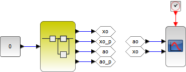
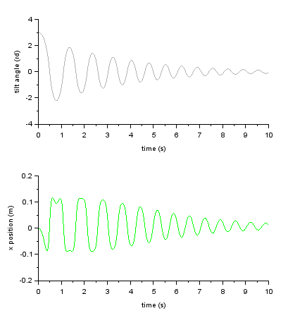
1.2.4. Simulation Results
The simulation represents a free fall of the pendulum, from the "almost" vertical starting point to the upside down position.
2. Linearization and Space-State representation
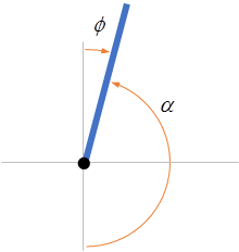
Linearization around the vertical position:
$\displaystyle\phi\approx{0}$
$\displaystyle\alpha=\pi+\phi$
$\displaystyle \sin{{\left(\alpha\right)}}= \sin{{\left(\pi+\phi\right)}}\approx-\phi$
$\displaystyle \cos{{\left(\alpha\right)}}= \cos{{\left(\pi+\phi\right)}}\approx-{1}$
Further assumptions:
$\displaystyle\dot{{\alpha}}^{2}\approx{0}$
$\displaystyle\eta\dot{{\alpha}}\approx{0}$
It comes:
First governing equation
| [7] → | $\displaystyle{\left({M}+{m}\right)}\ddot{{{x}}}+{b}\dot{{{x}}}-{m}{l}\ddot{{\phi}}={u}$ | [9] |
Second governing equation
| [8] → | $\displaystyle{\left({J}+{m}{l}^{2}\right)}\ddot{{\phi}}-{m}{g}{l}\phi-{m}{l}\ddot{{{x}}}={0}$ | [10] |
Solving [9] and [10] gives:
$\displaystyle\ddot{{{x}}}=\frac{{-{\left({J}+{m}{l}^{2}\right)}{b}\dot{{{x}}}+{\left({m}^{2}{g}{l}^{2}\right)}\phi+{\left({J}+{m}{l}^{2}\right)}{u}}}{{{J}{\left({M}+{m}\right)}+{M}{m}{l}^{2}}}$ | [11] |
$\displaystyle\ddot{{\phi}}=\frac{{-{\left({m}{b}{l}\right)}\dot{{{x}}}+{m}{g}{l}{\left({M}+{m}\right)}\phi+{\left({m}{l}\right)}{u}}}{{{J}{\left({M}+{m}\right)}+{M}{m}{l}^{2}}}$ | [12] |
And the corresponding Space State representation:
$\displaystyle{\left({\left.\begin{matrix}\dot{{{x}}}\\\ddot{{{x}}}\\\dot{{\phi}}\\\ddot{{\phi}}\end{matrix}\right.}\right)}={\left[{\left.\begin{matrix}{0}&{1}&{0}&{0}\\{0}&\frac{{-{\left({J}+{m}{l}^{2}\right)}{b}}}{{{J}{\left({M}+{m}\right)}+{M}{m}{l}^{2}}}&\frac{{{m}^{2}{g}{l}^{2}}}{{{J}{\left({M}+{m}\right)}+{M}{m}{l}^{2}}}&{0}\\{0}&{0}&{0}&{1}\\{0}&\frac{{-{\left({m}{b}{l}\right)}}}{{{J}{\left({M}+{m}\right)}+{M}{m}{l}^{2}}}&\frac{{{m}{g}{l}{\left({M}+{m}\right)}}}{{{J}{\left({M}+{m}\right)}+{M}{m}{l}^{2}}}&{0}\end{matrix}\right.}\right]}\times{\left({\left.\begin{matrix}{x}\\\dot{{{x}}}\\\phi\\\dot{{\phi}}\end{matrix}\right.}\right)}+{\left[{\left.\begin{matrix}{0}\\\frac{{{\left({J}+{m}{l}^{2}\right)}}}{{{J}{\left({M}+{m}\right)}+{M}{m}{l}^{2}}}\\{0}\\\frac{{{\left({m}{l}\right)}}}{{{J}{\left({M}+{m}\right)}+{M}{m}{l}^{2}}}\end{matrix}\right.}\right]}{u}$
$\displaystyle{\left({y}\right)}={\left[{\left.\begin{matrix}{1}&{0}&{0}&{0}\\{0}&{0}&{1}&{0}\end{matrix}\right.}\right]}\times{\left({\left.\begin{matrix}{x}\\\dot{{{x}}}\\\phi\\\dot{{\phi}}\end{matrix}\right.}\right)}+{\left[{\left.\begin{matrix}{0}\\{0}\end{matrix}\right.}\right]}{u}$
3. Control Synthesis
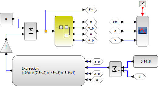
The linear optimal LQ full-state gain K is calculated using Scilab® 'lqr' function both in continuous and discrete time representations:
clear;
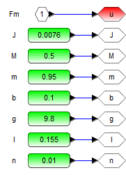
// Mechanical parameters
M = 0.5; // Mass of carriage (kg)
m = 0.95; // Mass of pendulum (kg)
b = 0.1; // Drag Coefficient (N/m/s)
I = 0.0076; // Pendulum Moment of Inertia (kg.m^2)
g = 9.8; // Gravity acceleration (m/s^2)
l = 0.155; // Half-length of pendulum (m)
//Space State Matrices
p = I*(M+m)+M*m*l^2;
A = [0, 1, 0, 0;
0, -(I+m*l^2)*b/p, (m^2*g*l^2)/p, 0;
0, 0, 0, 1;
0, -(m*l*b)/p, m*g*l*(M+m)/p, 0];
B = [0;
(I+m*l^2)/p;
0;
m*l/p ];
C = [1, 0, 0, 0;
0, 0, 1, 0];
D = [0;
0];
// *****************
// Contiunous domain
// *****************
// Define linear system in continuous domain
sbr_cont = syslin('c', A,B,C,D);
disp(sbr_cont);
// Print poles (showing instability)
disp(spec(A), "poles:");
// Check controlability
disp(rank(cont_mat(A,B)), "controlability matrix rank:");
// Check observability
disp(rank(obsv_mat(A,C)), "observability matrix rank:");
// Linear Quadratic control (lqr) effort
Q=diag([100,0,10,0]);
R = 1;
// Compute C1 and D12
[w,wp]=fullrf(sysdiag(Q,R));
C1=wp(:,1:4);
D12=wp(:,$:$);
// Compute correction matrix K
sbr_cont_k = syslin('c',A, B, C1, D12);
[K,X]=lqr(sbr_cont_k);
// Display new poles and K matrix
disp(spec(A+B*K), "new poles (continuous)");
disp(K,"K (continuous");
// Controlled system
Ac = [A + (B*K)];
Bc = [B];
Cc = [C];
Dc = [D];
// Set initial angle of 8°
X0 = [0; 0; -0.1416; 0]
// Defines controlled linear system
sbr_cont_ctrl = syslin('c', Ac, Bc, Cc, Dc, X0);
// ***************
// Discrete domain
// ***************
// Continuous -> Discrete
per = 0.05; // 50ms control loop
sbr_disc = dscr(sbr_cont,per);
disp(sbr_disc);
// Retreive matrices
A_d = sbr_disc(2);
B_d = sbr_disc(3);
C_d = sbr_disc(4);
D_d = sbr_disc(5);
// Check controlability
disp(rank(cont_mat(A_d, B_d)), "controlability matrix rank:");
// Check observability
disp(rank(obsv_mat(A_d, C_d)), "observability matrix rank:");
// Linear Quadratic control (lqr) effort
Q_d=diag([100,0,10,0]);
R_d = 1;
// Compute C1_d and D12_d
[w_d,wp_d]=fullrf(sysdiag(Q_d,R_d));
C1_d=wp_d(:,1:4);
D12_d=wp_d(:,$:$);
// Compute correction matrix K_d
sbr_disc_k = syslin('d',A_d, B_d, C1_d, D12_d);
[K_d,X_d]=lqr(sbr_disc_k);
// Display new poles and K matrix
disp(spec(A_d+B_d*K_d), "new poles (discrete)");
disp(K_d,"K (discrete)");
// Controlled discrete system
Ac_d = [A_d + (B_d*K_d)];
Bc_d = [B_d];
Cc_d = [C_d];
Dc_d = [D_d];
// Set initial angle of 8°
X0_d = [0; 0; -0.1416; 0]
// Defines controlled linear system
sbr_disc_ctrl = syslin('d', Ac_d, Bc_d, Cc_d, Dc_d, X0_d);
// **********
// Simulation
// **********
t = 0:per:4; // Time vector with 'per' resolution
sz = size(t);
r = zeros(1, sz(:,2)); // Input vector (no input)
y = csim(r,t,sbr_cont_ctrl); // Continuous model
pos = y(1,:);
tilt = y(2,:);
y_d = dsimul(sbr_disc_ctrl,r); // Discrete model
pos_d = y_d(1,:);
tilt_d = y_d(2,:);
figure(1);
clf(1);
subplot(2,1,1);
plot(t,pos_d, 'c.');
plot(t,pos,'b');
title('Cart Position');
xlabel('time (s)');
ylabel('position (m)');
subplot(2,1,2);
plot(t, tilt_d, 'm.')
plot(t,tilt,'k');
title('Pendulum tilt');
xlabel('time (s)');
ylabel('angle (rd)');
close(1);
The output of the script provides coefficients for the K matrix:
--> exec('D:\Users\Laurent\Documents\Projets\Segway\Simulation\segway_pomad.sce', -1)
!lss A B C D X0 dt !
0. 1. 0. 0.
0. -0.1356273 9.4726416 0.
0. 0. 0. 1.
0. -0.656432 93.278984 0.
0.
1.3562732
0.
6.5643197
1. 0. 0. 0.
0. 0. 1. 0.
0.
0.
0.
0.
0.
0.
c
poles:
0.
-0.0689621
-9.6917327
9.6250675
controlability matrix rank:
4.
observability matrix rank:
4.
new poles (continuous)
-9.6984204 + 1.1263055i
-9.6984204 - 1.1263055i
-1.9033796 + 1.7678988i
-1.9033796 - 1.7678988i
K (continuous)
10. 7.7757962 -43.074845 -5.120725
!lss A B C D X0 dt !
1. 0.0498292 0.0120455 0.0001993
0. 0.993111 0.490607 0.0120455
0. -0.0008347 1.1187499 0.0519645
0. -0.0339979 4.8392845 1.1187499
0.0017078
0.0688905
0.0083473
0.3399792
1. 0. 0. 0.
0. 0. 1. 0.
0.
0.
0.
0.
0.
0.
0.05
controlability matrix rank:
4.
observability matrix rank:
4.
new poles (discrete)
0.6148045 + 0.0350013i
0.6148045 - 0.0350013i
0.9056886 + 0.0803006i
0.9056886 - 0.0803006i
K (discrete)
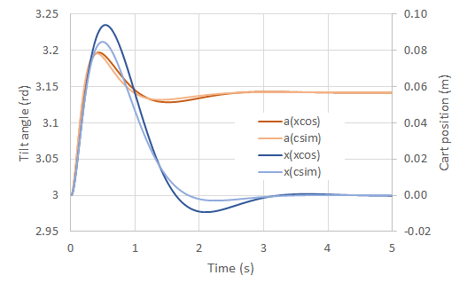
5.6181261 4.5784775 -31.721148 -3.6762483Simulation results show perfect matching between continuous and discrete-time models. In addition, K-matrix coefficients have been tried in the XCOS simulation together with the non-linear model of the Self-Balanced robot. Figure below compares the results obtained for both models and simulators when the robot is released with a small initial tilt angle. You can play with the Q matrix coef. The higher, the more feedback you get on the control, the more it costs in terms of power on the motors.
4. Motor and Wheels modeling
At first order, DC motor torque is proportional to the supplied current:
$\displaystyle{C}_{{{M}}}{\left({N}.{m}\right)}\approx\Phi\times{I}=\frac{{\Phi\times{V}_{{{M}}}}}{{{R}_{{{M}}}}}$
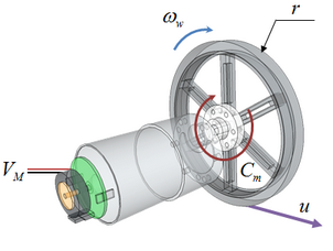
Summing the torque applied to the wheel gives:
$\displaystyle{J}_{{{W}}}\dot{{\omega}}_{{{W}}}={C}_{{{M}}}-{u}\times{r}$
The robot is assumed to be steady, so that regulation works around:
$\omega_{{{W}}}={0}$
$\dot{{\omega}}_{{{W}}}={0}$
It comes:
$\displaystyle{u}=\frac{{{C}_{{{M}}}}}{{{r}}}=\frac{{\Phi\times{V}_{{{M}}}}}{{{R}_{{{M}}}\times{r}}}$
Stalled motor resistance and torque/current relationship are provided by the motor manufacturer:
$\displaystyle{R}_{{{M}}}\approx{2.4}\Omega$
$\displaystyle\Phi\approx{1}\text{/}{8}{\left({N}.{m}.{A}^{{-{1}}}\right)}$
At first order, for r=5cm $\displaystyle{r}={5}{c}{m}$ , and taking account for the 2 wheels, we have almost u(N)=2*VM(V) $\displaystyle{u}{\left({N}\right)}={2}\times{V}_{{{M}}}{\left({V}\right)}$.
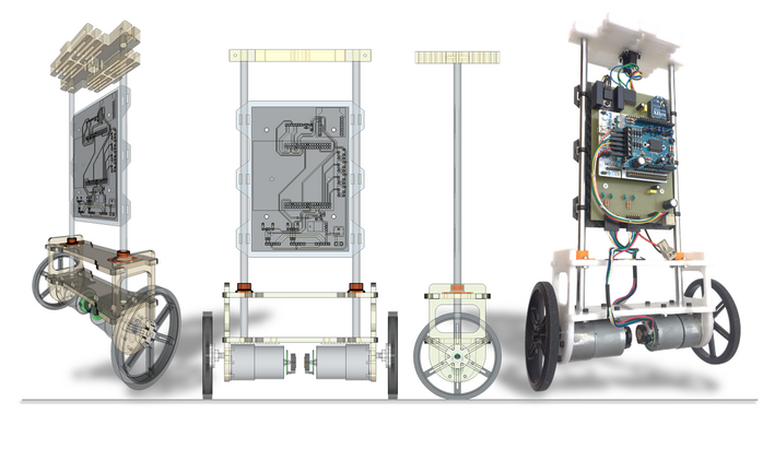
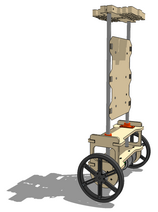
5. Fabrication resources
The robot is built by assembly of available boards:
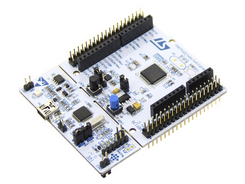
Nucleo F401RE for the CPU part
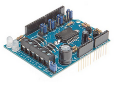
Arduino Motor Power Shield (fixed on the Nucleo)
Invensens MPU 9250 breakout board for the IMU
Everything is attached to a mother board screwed on the robot carbon vertical plate. The board includes a socket for RF module (BT, XBEE) to allow remote control.
You can get here the schematic of the mother board.
You can get here the mechanical design (Sketchup source model).
6. Embedded Software
The project archive contains a straightforward working code that keeps the robot (barely) steady.
- Log in to post comments