
3.6. Analog output DMA
1. Introduction
This tutorial will take you through the design of a sinewave signal generator. The basic idea is to output samples at regular time interval on the integrated Digital to Analog Converter (DAC) of the STM32F072 device.
Although samples could be calculated within the program itself by calling a sin() function available in the <math.h> library (as we did before), a different approach will be introduced here which is more efficient in terms of CPU usage.
The proposed method consists in storing a set (array) of pre-calculated output samples in the flash memory (beside the program itself), and then directly transferring these data with DMA from the memory to the DAC upon a Timer event which therefore defines the sampling period.
2. Building the wavetable
We need to store samples representing one single period of the signal we want to produce. Once a period has been generated, we can restart over the same array again and again to achieve a continuous sinewave generation.
A table of pre-calculated constants representing a function is called a Lookup Table. These can be used for a lot of purposes to avoid complex runtime maths and then save CPU with a price to pay in term of flash memory footprint.
For short tables of few samples you can compute the data manually and then edit the table. When the number of samples reaches a few tens, hundreds or even thousands samples, you'll want some scripts to generate the table automatically.
You can use anything you like to build your lookup tables. Here, we will make use of a Python script (the very same thing can be achieved with a Scilab®, Matlab®, Excel®...). Feel free to use what you're more comfortable with.

So, let's say that we want to pre-compute samples representing a single sinewave period with a resolution (step) of 6º, leading to a 360/6 = 60 samples table from 0° to 354° (360° being the same as 0°). The analog output comes from a 12-bit DAC which is fed with unsigned data ranging from 0 to 4095. We therefore need to center the sinewave sample around 211=2048. We also avoid extreme values to limit DAC analog buffer saturation issues by setting the amplitude to 2040.
Below is an example of Python script that generates such a sample table:
import numpy as np
import matplotlib.pyplot as plt

resolution = 6
offset     = 2048
amplitude  = 2040

# Compute number of sample
nsample     = int(360/resolution)
alpha       = np.linspace(0, (360-resolution), nsample)
sin_uint12  = np.round( ((np.sin(alpha*np.pi/180) * amplitude) + offset), 0 )

# Print output
print('Angle array')
print(alpha)
print('Sine samples (12-bit, unsigned)')
print(sin_uint12)

# Plot wavetable
fig = plt.figure(1)
fig.clf()
plt.title('Sine wavetable')
plt.xlabel('Alpha')
plt.ylabel('#')
plt.plot(alpha, sin_uint12, 'ro')
plt.xlim(0,360)
plt.xticks(np.arange(0, 360 +1, step=30))
plt.ylim(0,4096)
plt.yticks(np.arange(0, 4096 +1, step=256))
plt.grid(True)
plt.show()
Output is:
Angle array
[  0.   6.  12.  18.  24.  30.  36.  42.  48.  54.  60.  66.  72.  78.
  84.  90.  96. 102. 108. 114. 120. 126. 132. 138. 144. 150. 156. 162.
 168. 174. 180. 186. 192. 198. 204. 210. 216. 222. 228. 234. 240. 246.
 252. 258. 264. 270. 276. 282. 288. 294. 300. 306. 312. 318. 324. 330.
 336. 342. 348. 354.]

Sine samples (12-bit, unsigned)
[2048. 2261. 2472. 2678. 2878. 3068. 3247. 3413. 3564. 3698. 3815. 3912.
 3988. 4043. 4077. 4088. 4077. 4043. 3988. 3912. 3815. 3698. 3564. 3413.
 3247. 3068. 2878. 2678. 2472. 2261. 2048. 1835. 1624. 1418. 1218. 1028.
  849.  683.  532.  398.  281.  184.  108.   53.   19.    8.   19.   53.
  108.  184.  281.  398.  532.  683.  849. 1028. 1218. 1418. 1624. 1835.]
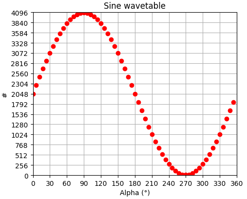
Notice that looping back from sample[59] to sample[0] perfectly joins for a continuous waveform.
You may also want to format the output to make the further copy/paste easier. You can for instance display data in a comma separated Hex format values with line jumps every 4 samples:
import numpy as np

resolution = 6
offset     = 2048
amplitude  = 2040

# Compute number of sample
nsample     = int(360/resolution)
alpha       = np.linspace(0, (360-resolution), nsample)
sin_uint12  = np.round( ((np.sin(alpha*np.pi/180) * amplitude) + offset), 0 )

# Print wavetable in HEX format
for k in range(nsample):
    h = '0x{:04x}'.format(int(sin_uint12[k]))
    print(h + ', ', end='')
    if ((k+1)%4 == 0):
        print()
Giving an output that is ready for copy/paste into the code editor:
0x0800, 0x08d5, 0x09a8, 0x0a76,
0x0b3e, 0x0bfc, 0x0caf, 0x0d55,
0x0dec, 0x0e72, 0x0ee7, 0x0f48,
0x0f94, 0x0fcb, 0x0fed, 0x0ff8,
0x0fed, 0x0fcb, 0x0f94, 0x0f48,
0x0ee7, 0x0e72, 0x0dec, 0x0d55,
0x0caf, 0x0bfc, 0x0b3e, 0x0a76,
0x09a8, 0x08d5, 0x0800, 0x072b,
0x0658, 0x058a, 0x04c2, 0x0404,
0x0351, 0x02ab, 0x0214, 0x018e,
0x0119, 0x00b8, 0x006c, 0x0035,
0x0013, 0x0008, 0x0013, 0x0035,
0x006c, 0x00b8, 0x0119, 0x018e,
0x0214, 0x02ab, 0x0351, 0x0404,
0x04c2, 0x058a, 0x0658, 0x072b,
For larger array you can even write the output directly into a file, but I'm not going into this here.
3. Prepare project
Create a new header file ![]() sinewave_table.h into your project under app/inc:
sinewave_table.h into your project under app/inc:
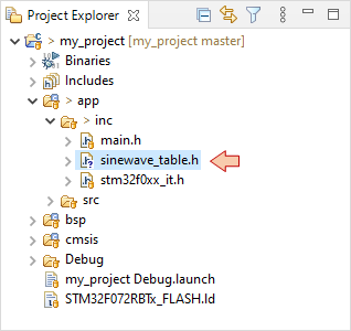
Open sinewave_table.h in the main editor and declare the sinewave[60] constant array using the above Python output. Take care of the very last ‘,’ that should be removed. By using the const type, the linker understands that data has to be stored in the flash memory (ROM) instead of RAM.
/*
 * sinewave_table.h
 *
 *  Created on: 14 juil. 2021
 *      Author: Laurent
 */

#ifndef INC_SINEWAVE_TABLE_H_
#define INC_SINEWAVE_TABLE_H_

/*
 * 60 samples Sine function wavetable
 * - 1 sample every 6°
 * - 12-bit unsigned scale
 */
const uint16_t sinewave[60] =
{
		0x0800, 0x08d5, 0x09a8, 0x0a76,
		0x0b3e, 0x0bfc, 0x0caf, 0x0d55,
		0x0dec, 0x0e72, 0x0ee7, 0x0f48,
		0x0f94, 0x0fcb, 0x0fed, 0x0ff8,
		0x0fed, 0x0fcb, 0x0f94, 0x0f48,
		0x0ee7, 0x0e72, 0x0dec, 0x0d55,
		0x0caf, 0x0bfc, 0x0b3e, 0x0a76,
		0x09a8, 0x08d5, 0x0800, 0x072b,
		0x0658, 0x058a, 0x04c2, 0x0404,
		0x0351, 0x02ab, 0x0214, 0x018e,
		0x0119, 0x00b8, 0x006c, 0x0035,
		0x0013, 0x0008, 0x0013, 0x0035,
		0x006c, 0x00b8, 0x0119, 0x018e,
		0x0214, 0x02ab, 0x0351, 0x0404,
		0x04c2, 0x058a, 0x0658, 0x072b
};

#endif /* INC_SINEWAVE_TABLE_H_ */
4. Peripherals setup
4.1. Timer setup
Let us first tune the timer time base configuration according the frequency we want for the output signal.
Having 60 samples to play for 1 signal period we can deduce:
$$f_{sample}=60\times f_{signal}$$
The frequency of timer update events is given by:
$$f_{update}=\frac{f_{sysclk}}{TIM_{prescaler}\times TIM_{period}}$$
Given that $f_{update}=f_{sample}$ we have:
$$f_{signal}=\frac{48MHz}{60\times TIM_{prescaler}\times TIM_{period}}=\frac{800kHz}{TIM_{prescaler}\times TIM_{period}}$$
The graph below plots the signal frequency $f_{signal}$ according to $TIM_{period}$ for various settings of $TIM_{prescaler}$.
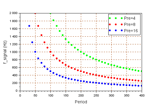
Let's say we want $f_{signal}=1kHz$. You can achieve that with many combinations of $TIM_{prescaler}\times TIM_{period} = 800$. Note that the lower the prescaler is, the more resolution you have around the desired frequency. Let us choose for instance:
$TIM_{prescaler} = 4$
$TIM_{period} = 200$
Edit the BSP_TIMER_Timebase_Init() function:
/*
 * BSP_TIMER_Timebase_Init()
 * TIM6 at 48MHz
 * Prescaler   = 4   -> Counting frequency is 12MHz
 * Auto-reload = 200 -> Update frequency is 60kHz
 */

void BSP_TIMER_Timebase_Init()
{
	// Enable TIM6 clock
	RCC->APB1ENR |= RCC_APB1ENR_TIM6EN;

	// Reset TIM6 configuration
	TIM6->CR1 = 0x0000;
	TIM6->CR2 = 0x0000;

	// Set TIM6 prescaler
	// Fck = 48MHz -> /4 = 12MHz counting frequency
	TIM6->PSC = (uint16_t) 4 -1;

	// Set TIM6 auto-reload register for 60kHz
	TIM6->ARR = (uint16_t) 200 -1;

	// Enable auto-reload preload
	TIM6->CR1 |= TIM_CR1_ARPE;

	// Enable Interrupt upon Update Event
	TIM6->DIER |= TIM_DIER_UIE;

	// Start TIM6 counter
	TIM6->CR1 |= TIM_CR1_CEN;
}
4.2. DAC setup
Leave the DAC initialization function as is it from previous tutorial:
/*
 * DAC_Init()
 * Initialize DAC for a single output
 * on channel 1 -> pin PA4
 */

void BSP_DAC_Init()
{
	// Enable GPIOA clock
	RCC->AHBENR |= RCC_AHBENR_GPIOAEN;

	// Configure pin PA4 as analog
	GPIOA->MODER &= ~GPIO_MODER_MODER4_Msk;
	GPIOA->MODER |= (0x03 <<GPIO_MODER_MODER4_Pos);

	// Enable DAC clock
	RCC->APB1ENR |= RCC_APB1ENR_DACEN;

	// Reset DAC configuration
	DAC->CR = 0x00000000;

	// Enable Channel 1
	DAC->CR |= DAC_CR_EN1;
}
5. Testing the signal generator
Now, edit the main() function:
...
#include "sinewave_table.h"
...

// Main function
int main()
{
	uint8_t		index;

	// Configure System Clock
	SystemClock_Config();

	// Initialize Console
	BSP_Console_Init();
	my_printf("Console Ready!\r\n");

	// Initialize 60kHz timebase
	BSP_TIMER_Timebase_Init();
	BSP_NVIC_Init();

	// Initialize DAC
	BSP_DAC_Init();

	// Initialize wavetable index
	index = 0;

	// Main loop
	while(1)
	{
		// Do every sampling period
		if(timebase_irq == 1)
		{
		    // Output a new sample
                    DAC->DHR12R1 = sinewave[index];

		    // Increment wavetable index
                    index++;
		    if (index==60) index = 0;

		    // Reset timebase flag
		    timebase_irq = 0;
		}
	}
}
Build the project and flash the target.
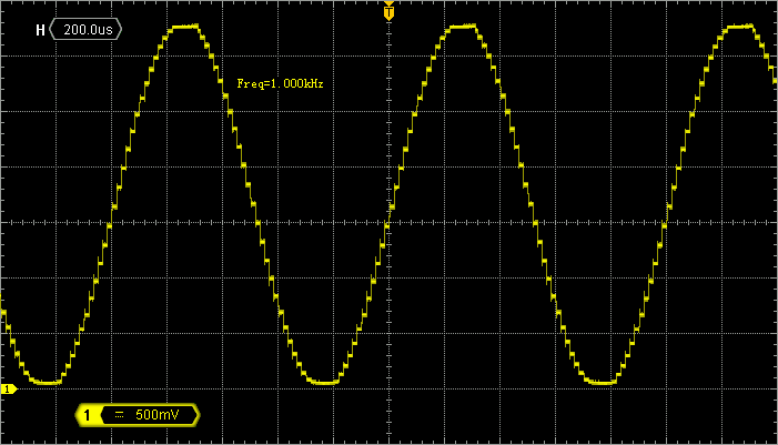
You can now probe the PA4 pin with an oscilloscope. You should see the 3.3Vpp sinewave generated at 1kHz.
 | - - |
6. Releasing CPU load
Can we do the same thing without CPU intervention? Guess what... the answer is Yes!
6.1. DAC setup with DMA and Timer triggering
Edit the BSP_DAC_Init() function. What we need to add is:
A DMA configuration for Channel 3 that automatically conveys samples from the sine wavetable to the DAC output register. It is similar to what has been done before, but note that for the first time we want a Memory→Peripheral transfer direction
Enable the DAC DMA request, of course
A synchronous mechanism that triggers DAC output (and therefore DMA requests) based on TIM6 update event, without CPU intervention. This is achieved by using TRGO internal signal that directly connects TIM6 to the DAC.
/*
 * DAC_Init()
 * Initialize DAC for a single output
 * on channel 1 -> pin PA4
 */

extern const uint16_t sinewave[60];

void BSP_DAC_Init()
{
	// Enable GPIOA clock
	RCC->AHBENR |= RCC_AHBENR_GPIOAEN;

	// Configure pin PA4 as analog
	GPIOA->MODER &= ~GPIO_MODER_MODER4_Msk;
	GPIOA->MODER |= (0x03 <<GPIO_MODER_MODER4_Pos);

	// Enable DMA clock
	RCC->AHBENR |= RCC_AHBENR_DMA1EN;

	// Reset DMA1 Channel 3 (DAC) configuration
	DMA1_Channel3->CCR = 0x00000000;

	// Configure DMA1 Channel 3
	// Memory -> Peripheral
	// Peripheral is 16-bit, no increment
	// Memory is 16-bit, increment
	// Circular mode

	DMA1_Channel3->CCR |= (0x01 <<DMA_CCR_PSIZE_Pos) | (0x01 <<DMA_CCR_MSIZE_Pos) | DMA_CCR_MINC | DMA_CCR_CIRC | DMA_CCR_DIR;

	// Peripheral is DAC1 DHR12R1
	DMA1_Channel3->CPAR = (uint32_t)&DAC1->DHR12R1;

	// Memory is sine wavetable
	DMA1_Channel3->CMAR = (uint32_t)sinewave;

	// Set Memory Buffer size
	DMA1_Channel3->CNDTR = 60;

	// Enable DMA1 Channel 3
	DMA1_Channel3->CCR |= DMA_CCR_EN;

	// Enable DAC clock
	RCC->APB1ENR |= RCC_APB1ENR_DACEN;

	// Reset DAC configuration
	DAC->CR = 0x00000000;

	// Enable DAC Channel 1 DMA request
	DAC->CR |= DAC_CR_DMAEN1;

	// Select and enable TIM6 TRGO event as DAC trigger source
	DAC->CR |= (0x00 <<DAC_CR_TSEL1_Pos) | DAC_CR_TEN1;

	// Enable Channel 1
	DAC->CR |= DAC_CR_EN1;
}
6.2. Timer setup for autonomous DAC synchronization
We then need to enable TIM6 TRGO output trigger based on update events. You may also disable TIM6 interrupt by commenting the corresponding line as we want to demonstrate that CPU is not involved in the process:
/*
 * BSP_TIMER_Timebase_Init()
 * TIM6 at 48MHz
 * Prescaler   = 4   -> Counting frequency is 12MHz
 * Auto-reload = 200 -> Update frequency is 60kHz
 */
void BSP_TIMER_Timebase_Init()
{
	// Enable TIM6 clock
	RCC->APB1ENR |= RCC_APB1ENR_TIM6EN;

	// Reset TIM6 configuration
	TIM6->CR1 = 0x0000;
	TIM6->CR2 = 0x0000;

	// Set TIM6 prescaler
	// Fck = 48MHz -> /4 = 12MHz counting frequency
	TIM6->PSC = (uint16_t) 4 -1;

	// Set TIM6 auto-reload register for 60kHz
	TIM6->ARR = (uint16_t) 200 -1;

	// Enable auto-reload preload
	TIM6->CR1 |= TIM_CR1_ARPE;

	// Enable Interrupt upon Update Event
	// TIM6->DIER |= TIM_DIER_UIE;

	// Enable TRGO on update event
	TIM6->CR2 |= (0x02 <<TIM_CR2_MMS_Pos);

	// Start TIM6 counter
	TIM6->CR1 |= TIM_CR1_CEN;
}
6.3. Testing the setup
Edit the main() function so that CPU is held into an infinite empty loop, after everything has been initialized:
...

// Main function
int main()
{
	// Configure System Clock
	SystemClock_Config();

	// Initialize 60kHz timebase
	BSP_TIMER_Timebase_Init();

	// Initialize DAC
	BSP_DAC_Init();

	// Main loop
	while(1)
	{
		// Do nothing...
	}
}
You can now try and run the project. The CPU is doing absolutely nothing and still, if you probe PA4 you should get a nice 1kHz sine wave output.
Note that there is no need of pointer in the wavetable, and that there is no interruption involved in the process (NVIC is even not initialized).
To make ideas even clearer, launch a debug session ![]() and step over
and step over ![]() initialization code while watching the oscilloscope. You’ll see the sine wave appearing as soon as you’ve step over the DAC initialization function, even with CPU halted by the debugger.
initialization code while watching the oscilloscope. You’ll see the sine wave appearing as soon as you’ve step over the DAC initialization function, even with CPU halted by the debugger.
Isn't that Cool?
| - - |
7. A little more on sampled waveforms…
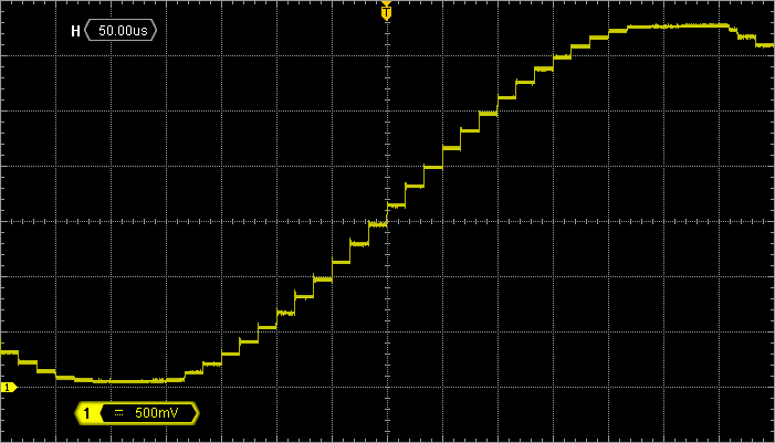
Taking 60 samples per signal period produces a pretty smooth sinewave signal, although you can see the discrete samples quite well on the oscilloscope:
You may (or may not) know that the sampling process produces noise and harmonic distortion because of the discretization process of both time (sampling period) and amplitude (DAC resolution) scales.
7.1. A bit of theory
A common approach to measure noise and harmonic distortion of a signal is to analyze its spectrum. A signal spectrum represents the distribution of the signal power along the frequency axis. For this reason, we call “frequency-domain” such a signal representation. It differs from the classical “time-domain” representation you get from the oscilloscope.
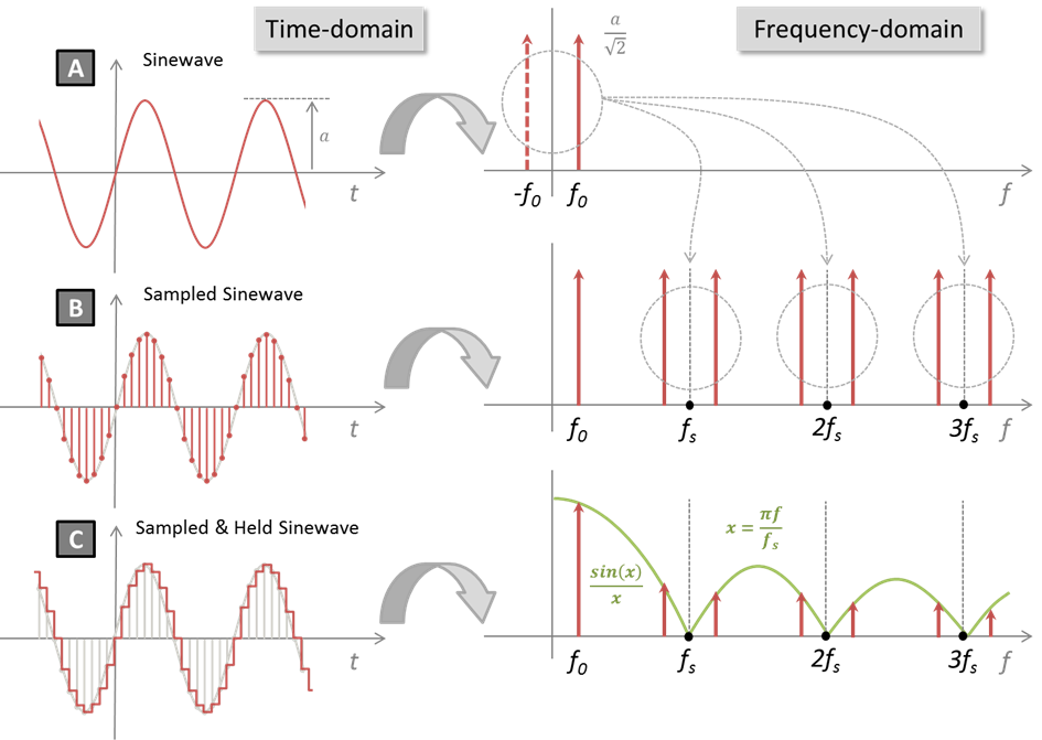
For a pure sinusoidal signal, all the power is concentrated on a single frequency which is the signal frequency ($f_0$ in the figure below). Therefore, the spectrum exhibits a single frequency compound $f_0$. The amplitude of this compound corresponds to the RMS value of the sinusoidal signal. This is shown in the figure below (A). Note that although we usually represent only the positive side of the frequency axis, a negative side also exists, mirroring the positive side of the spectrum.
The sampling process is described in situation (B) where the sinewave is only observed at uniformly spaced points in time. Just like snapshots. Doing this produces duplicates (or images) of the original spectrum (including its negative compound) at every multiples of the sampling period $f_s$.
Nevertheless, signal (B) is not the one we can see on the oscilloscope. In practice, the DAC is holding (maintaining) a sample value during a whole sampling period and until a new sample is available. Therefore, the signal is not only sampled, it is also held. This corresponds to situation (C). In that case, the whole spectrum of (B) is multiplied in amplitude by a cardinal sine function (sinc), which mostly attenuates the spectrum's images.
Another important theoretical result concerns the noise resulting from the quantization process in amplitude (i.e. discrete values of the DAC output). In the case of an ideal DAC, one can demonstrate that the SNR (Signal-to-Noise Ratio) integrated over a bandwidth between DC and fs/2 cannot be better than:
$$SNR=6.02N+1.76dB$$
where N is the number of bits available with the DAC. In our case, with N=12, we have:
$$SNR_{12bit}=74dB$$
Note that this is a purely theoretical limit, with ideal DAC and no other noise source than the quantization process. In practice, we always measure inferior SNR. Better SNR can still be obtained over a reduced bandwidth (i.e. using a low-pass filtering). That's what you get when you hit the ‘average’ button of the oscilloscope...
7.2. A bit of practice
If you have an oscilloscope with the FFT (Fast Fourier Transform) capability (any oscilloscope nowadays) you can turn this function on. Also set the input signal channel to AC coupling in order to remove the Vdd/2 offset from the analysis.
FFT is a digital algorithm that takes time domain data as input (i.e. signals on oscilloscope channels) and compute frequency-domain data as output (i.e. spectrum). Try to play with the settings (mostly time and amplitude scales). If you are good enough, you may get this:
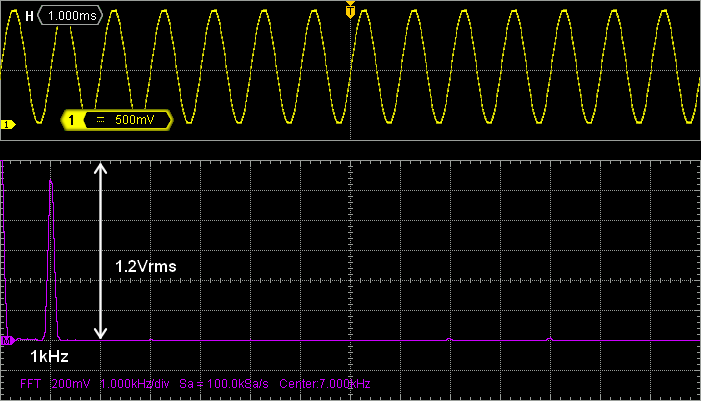
The main frequency compound is found at 1kHz (as expected) with an amplitude of about 1.2Vrms which corresponds to:
$$A_0=\frac{V_{dd}/2}{\sqrt{2}}=1.16V_{rms}$$
Signal theory told us that the spectrum of the signal, when sampled, is imaged around each multiple of the sampling frequency. The sampling frequency in the tutorial was:
$$f_s=f_{update}=\frac{f_{sysclk}}{TIM_{prescaler}\times TIM_{period}}=\frac{48MHz}{4\times 20}=60kHz$$
In the screenshot above, with 1kHz/div on the FFT, the first spectrum replica at 60kHz is far on the right, beyond screen. Changing oscilloscope and FFT range reveals the expected first harmonic images around 60kHz, and 120kHz…

Focus on the spectrum around 60kHz. We have:
The image of the negative part of the ideal sinewave at $f_s-f_0=59kHz$
The image of the positive part of the ideal sinewave at $f_s+f_0=61kHz$
We can compute the sinc function for each of these frequencies considering :
$$x=\frac{\pi f}{f_s}$$
$$\frac{sin\, x}{x} (@59kHz)= 16.9\times10^{-3})$ → $A_1\approx1.16\times16.9\times10^{-3} = 19.6mV$$
$$\frac{sin\, x}{x} (@61kHz)= 16.4\times10^{-3})$ → $A_2\approx1.16\times16.4\times10^{-3} = 19 mV$$
If you look at the amplitude measured in the above screenshot (vertical grid unit is 5mV), you will see a very good match with these theoretical results. Do the same around 120kHz, you will get a good match again with amplitude close to 10mV.
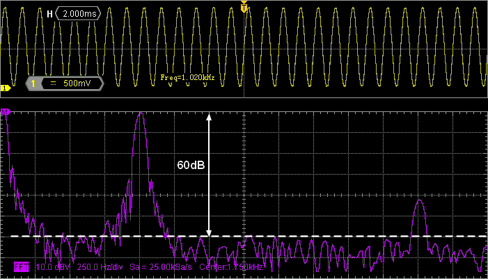
Regarding SNR, you can get an idea by using the dB scale of FFT. SNR is the distance between the fundamental peak height and the noise floor. Here, it is close to 60dB. This is equivalent to the ideal SNR obtained with a 10-bit discretization process.
Let us now make things bad, for fun…
Instead of having 60 samples per signal period, we build a new wavetable with only 8 samples (i.e. a sample every 45°):
const uint16_t sinewave_lowres[8] =
{
		0x0800, 0x0da2, 0x0ff8, 0x0da2,
		0x0800, 0x025e, 0x0008, 0x025e
};
/*
 * DAC_Init()
 * Initialize DAC for a single output
 * on channel 1 -> pin PA4
 */

extern const uint16_t sinewave[60];
extern const uint16_t sinewave_lowres[8];

void BSP_DAC_Init()
{
	...

	// Memory is sine wavetable
	DMA1_Channel3->CMAR = (uint32_t)sinewave_lowres;

	// Set Memory Buffer size
	DMA1_Channel3->CNDTR = 8;

	...
}
Leaving the timer's settings as they are, we still have a sampling frequency of 60kHz, but now the signal frequency becomes:
$$f_{signal}=\frac{48MHz}{8\times TIM_{prescaler}\times TIM_{period}}=\frac{60kHz}{8}=7.5kHz$$
In this situation, spectrum replicas every 60kHz are quite noticeable with an amplitude of ≈150mVrms for the first one:
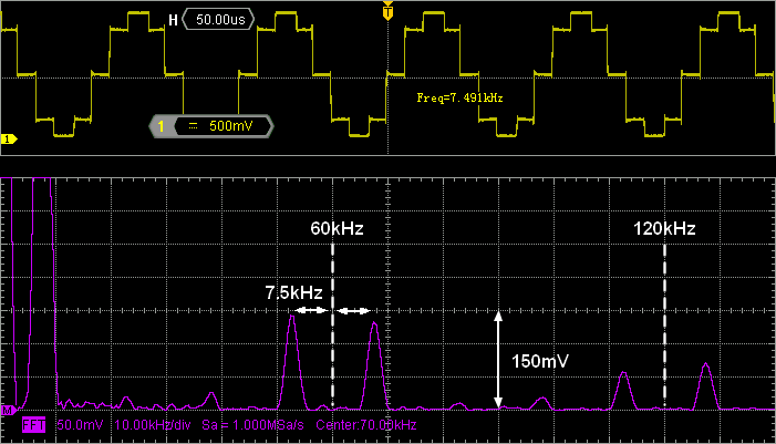
Again, let us verify this result:
$$\frac{sin\, x}{x} (@52.5kHz)= 139\times10^{-3})$ → $A_1\approx1.16\times139\times10^{-3} = 161mV$$
$$\frac{sin\, x}{x} (@67.5kHz)= 108\times10^{-3})$ → $A_2\approx1.16\times108\times10^{-3} = 125mV$$
Good match again!
Signal theory is a wide topic that we are not going to cover here. At this point, it is just important that you get a basic feeling of what the sampling process involves in terms of harmonic distortion. The ratio between sampling frequency and signal frequency (i.e. the number of sample per signal period) is a determinant factor to pay attention to in order to reduce the distortion produced by the sampling process.
8. Summary
In this tutorial, you have learned how to output sample from the DAC without any load on the CPU by making a clever use of both DMA and timer TRGO capability.
- Log in to post comments