1.4. Sensitivity & Monte Carlo Analysis

Introduction

At some point, you'll be able to design analog circuit to fulfill given specifications. The question that arises next is Is my design robust enough?

Robust to what?

Robustness is expressed against design parameters that are subject to variability. Variability in electrical engineering commonly relates to:

• Process variability, representing uncertainties inherent to the fabrication process. In this category, we'll find the uncertainties associated to component values (e.g. a resistor value, a transistor current gain, ...). These are provided by part manufacturers.

• Voltage variability, representing the possible change in supply voltage. For instance a 1S Li-Ion battery powered system should work the same from 4.2V (full-charge) down to 3.5V (empty).

• Temperature variability, representing effects of environmental conditions. We know for instance that resistors are temperature sensitive, but also transistors.

This tutorial addresses the first category of uncertainties. To better illustrate the matter, I'll use the well-known Sallen-Key implementation of 2nd order band-pass filter.

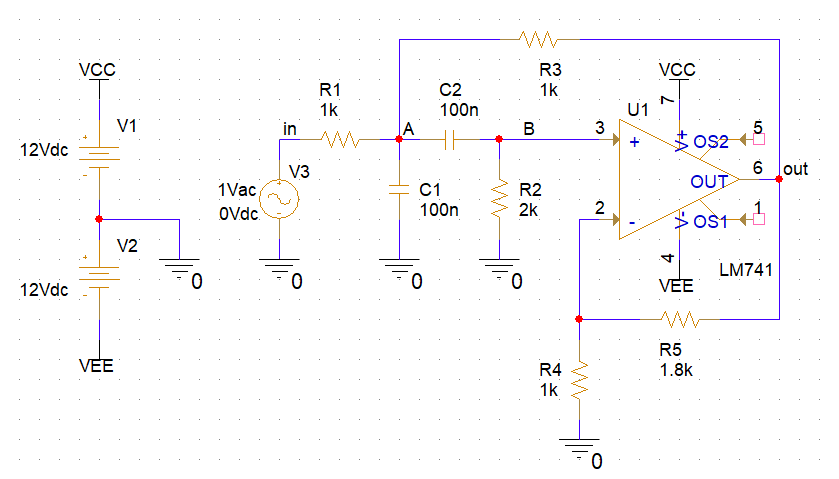
Within Capture , you may start a new project (e.g. 'tuto_sk') and edit the following schematic. Make sure to use PSpice-only libraries.

1. Analytical study - Part I (simplified version)

1.1. Transfer function

The simplified transfer function can be easily obtained if one assumes the following conditions:

• $R_1$ = $R_3$ = $R$

• $R_2$ = $2R$

• $C_1$ = $C_2$ = $C$

In addition, let us writes:

$R_5 = R_4(A_v-1)$

With $A_v = 1+\frac{R_5}{R_4}$ the gain of the non-inverting amplifier stage.

The voltage gain across the amplifier stage gives:

$$v_{out} = {A_v} {v_B}$$

With voltage at node B given by:

$$v_B = v_A\frac{2RCp}{1+(2RCp)}$$

Now, summing current at node A, we have:

$$\frac{v_{in}-v_A}{R}+\frac{v_{out}-v_A}{R}+{(v_B-v_A)}Cp-v_ACp=0$$

Solving the above equations finally gives the second order band-pass tranfer function:

$$\frac{v_{out}}{v_{in}}=\frac{A_v\, R C p}{1+\left( 3-A_v\right)  R C p+{{R}^{2}}\, {{C}^{2}}\, {{p}^{2}}}$$

The general second order band-pass transfer function is given by:

$$H(p)=G\frac{\frac{2m}{\omega_0}p}{1+\frac{2m}{\omega_0}p+\frac{p^2}{\omega_0^2}}$$

So that:

$$\omega_0=\frac{1}{RC}$$

$$m = \frac{(3-A_v)}{2}\rightarrow Q=\frac{1}{2m}=\frac{1}{(3-A_v)}$$

$$G=\frac{A_v}{(3-A_v)}$$

According the above schematic design values, we have :

• $\omega_0=10^4 rad/s \rightarrow f_0 = 1.59kHz$

• $Q = 5$

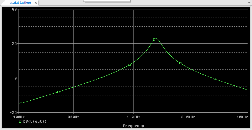
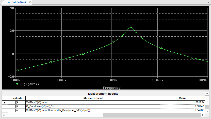
This is confirmed by AC analysis:

1.2. Sensitivity

The sensitivity relates desirable characteristics of a circuit (i.e. gain, bandwidth, cutoff frequencies, quality factor, input and output impedance...) to parameter variations (e.g. component values).

The sensitivity analysis basically computes a gain between a chosen characteristic and a chosen parameter. For instance in the above example, it would be interesting to express the dependency of the cutoff frequency $f_0$ with respect to the value of the resistor R.

Well, this can be simply archived by differentiating the expression of $f_0$ with respect to R:

$$f_0=\frac{1}{2\pi RC}$$

$$\frac{\partial f_0}{\partial R}=\frac{-1}{2\pi R^2C}\,(Hz/\Omega)$$

With $R=1k\Omega$ anc $C=100nF$, we get a frequency shift of $-1.59Hz$ for an increase of $1\Omega$ in R. The previous expression provides an absolute sensitivity (in $Hz/\Omega$). Yet, a change in resistor value is better expressed relatively to its nominal value (in %) the same way the manufacturer specifies its tolerance range.

The above derivative can be rewritten:

$$\partial f_0=\left (\frac{-1}{2\pi R^2C}\right )\times \left (\frac{\partial R}{ R}\right )\times R=\left (\frac{-1}{2\pi RC}\right )\times \left (\frac{\partial R}{ R}\right )$$

Then, a change of $10\Omega$ from $R_{nom}=1k\Omega$ corresponds to a $1\%$ change in the resistor value and produces a shift of $15.9Hz$ in the cutoff frequency. The sensitivity of cutoff frequency with respect to a relative change in $R$ writes:

$$\frac{\partial f_0}{(\frac{\partial R}{ R})_{\%} }=\left (\frac{-1}{2\pi RC}\right )\times \frac{1}{100}$$

Let's take another example. In the above case study, we established that the quality factor Q only depends on the gain Av:

$$Q=\frac{1}{2m}=\frac{1}{(3-A_v)}$$

$$\frac{\partial Q}{\partial A_v}=\frac{1}{{{\left( 3-A_v\right) }^{2}}}$$

$$\frac{\partial Q}{Q}=\frac{\partial A_v}{A_v}\times\frac{\partial Q}{\partial A_v}\times \frac{A_v}{Q}=\frac{\partial A_v}{A_v}\times \frac{1}{(3-A_v)^2}\times A_v(3-A_v)$$

$$\frac{\partial Q}{Q}=\frac{\partial A_v}{A_v}\times A_v Q$$

The above result shows that if you want to keep Q within (for instance) a $10\%$ error, you need to keep the error on the gain $A_v$

• below $5\%$ with $Q=1$

• below $2\%$ with $Q=2$

• below $0.7\%$ with $Q=5$

Considering that $A_v$ depends on two resistors with given tolerance, you can guess that keeping control on high quality factor is raher difficult.

2. Analytical study - Part II (full version)

Yet, the above results are not really meaningful. As a matter of fact $R$ does not exist. $R$ comes from an assumption that all 3 resistors in the upper part of the schematic ($R_1$,$R_2$,$R_3$) are well matched, which is not the case in the real life. The same applies to $C$. $A_v$ does exist, but it results from the assembly of two resistors $R_4$ and $R_5$.

Therefore, a valid theoretical sensibility study cannot assume component matching (unless they really are), and must consider each part independency in the filter transfer function. The 'true' Sallen-Key band-pass filter transfer function is given below. Trust me, and thank you maxima!

$$\frac{v_{out}}{v_{in}}=\frac{\frac{A_v C_2 R_2 R_3}{R_1+R_3} p}{\left(\frac{R_1 R_2 R_3 C_1 C_2}{R_1+R_3}\right)  p^2+\left(\frac{R_3 (R_2 C_2 + R_1 (C_1+C_2)  ) + (1-A_v) R_1 R_2 C_2}{R_1+R_3} \right)  p+ 1)}$$

From there, we can identify circuit characteristics:

$$\omega_0 = \sqrt{\frac{{R_1}+{R_3}}{{R_1} {R_2} {R_3}{C_1} {C_2}}}$$

$$Q=\frac{{R_3}+{R_1}}{\sqrt{\frac{{R_3}+{R_1}}{{C_1} {C_2} {R_1} {R_2} {R_3}}}\left( \left( {C_2} {R_2}+\left( {C_2}+{C_1}\right)  {R_1}\right)  {R_3}-\frac{{C_2} {R_1} {R_2} {R_5}}{{R_4}}\right) }$$

And then proceed to derivation. We consider for example the sensitivity of $\omega_0$ to variations of $R_1$ and $R_2$:

$$\frac{\partial \omega_0}{\partial R_1}=-\frac{1}{2 {C_1} {C_2} {{{R_1}}^{2}} {R_2} \omega_0}$$

$$\frac{\partial \omega_0}{\partial R_2}=-\frac{{R_3}+{R_1}}{2 {C_1} {C_2} {R_1} {{{R_2}}^{2}} {R_3} \omega_0}$$

Once the literal expression of each derivative is found, we may re-introduce our nominal case of resistors and capacitor matching:

$$\frac{\partial \omega_0}{\partial R_1}=\frac{\partial \omega_0}{\partial R_2}=-\frac{1}{4 R^3 C^2  \omega_0}$$

The frequency shift is therefore $-2.5(rd/s)/\Omega$ or $-0.4Hz/\Omega$ for both $R_1$ and $R_2$.

We can also compute the sensitivity of the quality factor $Q$ with respect to $R_5$ and $R_4$ the same way:

$$\frac{\partial Q}{\partial R_5}=\frac{1}{\omega_0 {R^2C(3-A_v)^2}}$$

$$\frac{\partial Q}{\partial R_4}=-\frac{ {R_5}} {\omega_0 RC R_4^2 (3-A_v)^2}$$

It results in a sensitivity of $25.10^{-3}/\Omega$ for $R_5$ and $-45.10^{-3}/\Omega$ for $R_4$. All the above are absolute sensitivities.

3. Using Cadence Advanced Analysis

3.1. Sensitivity Analysis

Step 1: Setting up measurements

There are several pre-defined measurements you can perform on a simulation result. A measurement results in a scalar value extracted from a regular PSpice analysis : DC Sweep, TRAN or AC.

In our case study, both cutoff frequency and quality factor relate to the frequency response of the circuit, and hence to an AC analysis. Because measurement are sensitive to the simulation resolution, let us first tune our simulation settings to provide high resolution in the region of interest (i.e. in the vicinity of 1.6kHz):

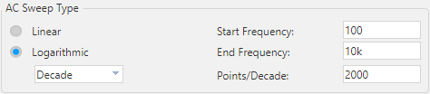
2000 points per decade seems quite a lot, but we'll see that fine resolution is important for the (coming soon) sensitivity analysis.

Run the AC Analysis , then in the PSpice result window, plot the magnitude Bode diagram as shown above.

Once you've got the expected frequency response, click the Evaluate Measurements button or use the Trace menu entry in the PSpice Simulator window. Then you'll be able to construct measurement expressions. We basically want to automate the measurement of both the cutoff frequency and the quality factor of the filter.

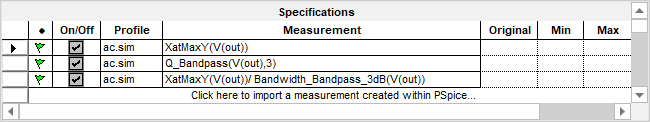
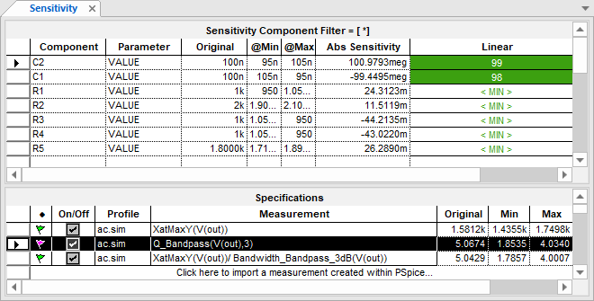
• For the cutoff frequency, which corresponds to frequency giving the maximum gain in the simulation we may use: 'XatMaxY(V(out))'.
  
  
   

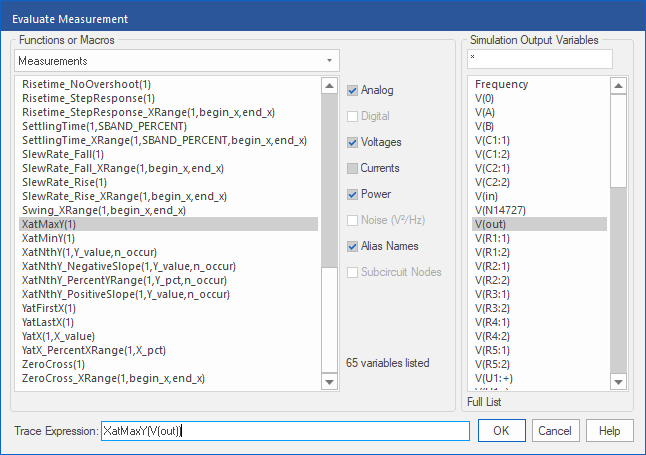
• For the quality factor, there's a ready-to-use macro: 'Q_Bandpass(V(out),3)'.
  
  You may also use the definition of the quality factor $Q=\frac{f_0}{BW}$ and construct 'XatMaxY(V(out))/ Bandwidth_Bandpass_3dB(V(out))' expression. Both should be valid and provide about the same result.

You'll end up with something similar to this:

Well done. You may keep the PSpice Simulator window open, but for now let go back to the schematic.

Step 2: Tolerance assignment

From the main Capture window, click the Assign tolerance for Advanced Analysis button . You get a dialog interface to setup each part uncertainty.

Select each passive component ($R_1$, $R_2$, $R_3$, $R_4$, $R_5$, $C_1$, $C_2$) one by one and set the relative tolerance to $\pm5\%$ with a Gaussian distribution. Below is an example with $C_2$:

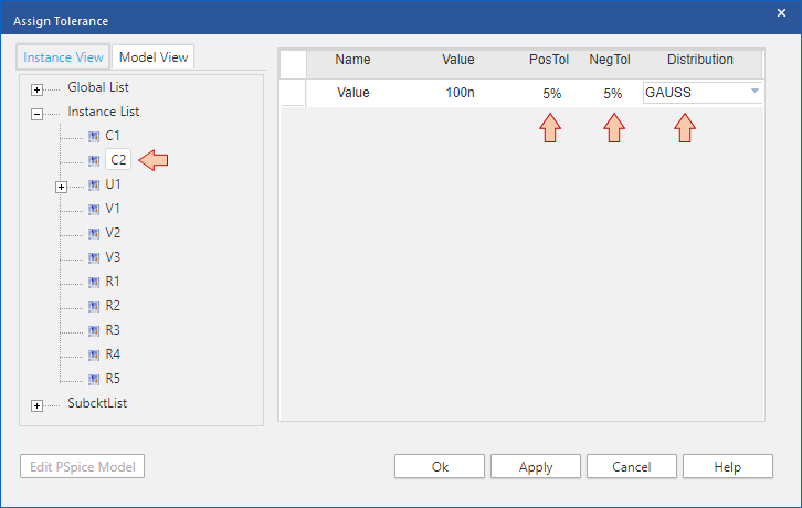
When you're done click Apply and then OK.

Step 3: Running Sensitivity Analysis

Click the Start Advanced Analysis - Sensitivity button .

The AMS Advanced Analysis dialog takes few seconds to open. Hopefully, you'll get the interface shown below. Make sure the main toolbar displays 'Sensitivity' and that the entire list of passive parts (the exact ones with tolerance assignments) is on display.

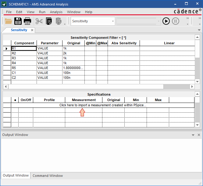
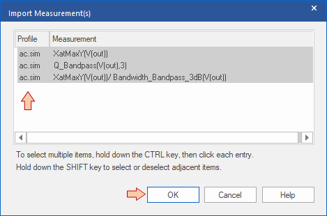
Click on the measurement import field. If you've done right until now, you should retrieve the measurements you've setup within the AC simulation profile. Select all and then click OK.

The Specifications table is updated:

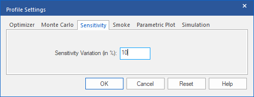
Finally, enter the Edit→Profile Settings menu. In the Sensitivity tab, set the Sensitivity Variation to 10% and click OK.

You may wonder what's this for...

Well (deep breathing...), in a sensitivity analysis, the parameter variation (e.g. resistor value) is our "small signal" input, the output being the characteristic of interest (e.g. the cutoff frequency). That was the case above when we established partial derivative. These derivative assume a linear system, which is most likely not the case. The sensitivity analysis works the same. It calculates partial derivatives based on two simulation points. One corresponds to the nominal case, the second being calculated by shifting the targeted parameter some 'amount' in the positive direction. What Sensitivity Variation sets is precisely that 'amount'. It is given in unit of % of the tolerance % you've set before. Doing so, we can compute partial derivatives using a small amount of parameter variation and then get a better match with analytical derivatives established before (i.e. a better local slope). Larger parameter variation may lead to wrong sensitivity results.

But (deep breathing again...), in some cases, a too low parameter variation may produce no result at all. That's very much likely if your simulation profile (AC analysis here) is not detailed (x-axis, frequency resolution) enough. That's the very reason why we asked for a 2000 points/decade computing resolution.

Once a given partial derivative has been computed using tiny variations, result is linearly extrapolated to the full tolerance range of the corresponding parameter.

In summary, be careful with this setting and try for yourself. Keep in mind that results strongly depends on the various settings you've done both in the simulation profile, and here. Review results carefully.

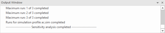
You may now run the Sensitivity Analysis. Just click button and watch le log area.

Step 4: Reviewing Results

When simulation completes you can browse results.

Below are the results regarding the $f_0$ absolute sensitivity. With $-0.36Hz/\Omega$ for both $R_1$ and $R_2$, we've got a pretty good mach with the theoretical result of $-0.4Hz/\Omega$ established previously.

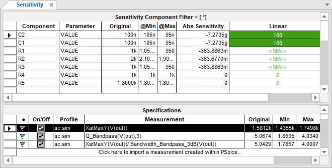
Next is the Q sensitivity. Again, numerical results of $26.10^{-3}/\Omega$ for $R_5$ and $-43.10^{-3}/\Omega$ for $R_4$ are in very good agreement with theoretical results ($25.10^{-3}/\Omega$ for $R_5$ and $-45.10^{-3}/\Omega$ for $R_4$).

Obviously, absolute sensitivities for capacitors are huge because the unit is $/Farad$ ! Moreover, absolute sensitivities do not really tell which parts you need to keep under control most. You better use the relative sensitivity view for that.

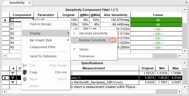
Right-click in the result area and select the Relative Sensitivity display:

Much better! It reveals that the value of $R_5$ is the most 'controlling' parameter of the Q factor. This is not really a surprise. On the contrary, values of $C_1$ and $C_2$ do not affect Q that much.

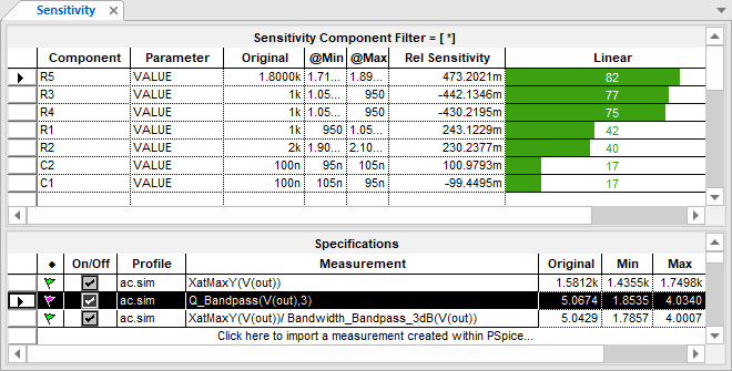
Note that the relation between absolute et relative sensitivity is simply:

$$REL_{sensitivity}=ABS_{sensitivity}\times \frac{P_{nominal}}{100}$$

Where $P_{nominal}$ is the parameter nominal value.

3.2. Monte Carlo Analysis

The Monte Carlo Analysis is very important in the analog design field. No analog IC design is sent for fabrication before passing this check point.

The Monte Carlo analysis is a statistical approach that 'simulate' the batch fabrication of many circuits by generating several 'unique' sample circuits. For each sample, parameters value are randomly chosen within their specified distribution (i.e. within tolerance range). This is representative of the process variability in a production environment.

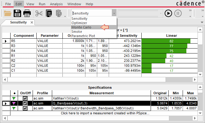
You may switch to Monte Carlo analysis directly from the Advanced Analysis environment, or if it is closed, from the main windows using the button.

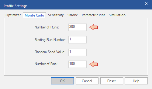
Open Edit→Profile Settings and tune the Monte Carlo simulation as follows. The number of runs (i.e. simulated samples) must be large enough to be representative, but the more you put here, the longer it takes to compute. The number of bins refers to the histogram view of the results.

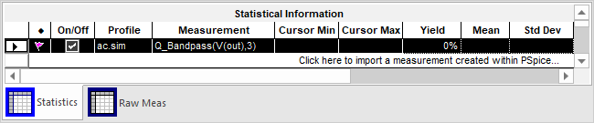
Import the Q factor measurement in the measurement field, the same way you did with the sensitivity analysis:

Run the simulation and watch out the log area. It takes a couple of minutes because we're running the AC analysis 200 times. When the simulation completes, you get a histogram view representing the distribution of the 200 'simulated' sample circuits with respect the characteristic of interest (Q factor here).

You can see that only few circuits among 200 perfectly match the targeted Q=5. Summing the two closest bins we barely reach a total 35 circuits.

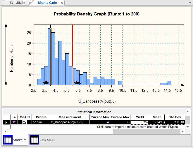
You can play with the graph area (zoom in/out) and place Min & Max bars. Let say for instance that we want to produce tons of Sallen-Key filters, and that our specification regarding Q factor is between 4 and 6 (i.e. Q factors outside this range cannot be sold).

With actual design, and actual components tolerance we can only sell 53% of the circuits coming out the production chain (Yield). In other words, about half the production goes to the trash can, although our design works wonderfully with nominal case.

Now, you see how important this is?

Well, let us buy more expensive parts with 1% tolerance range instead of the regular 5% set before:

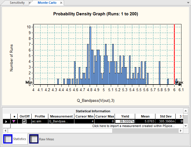
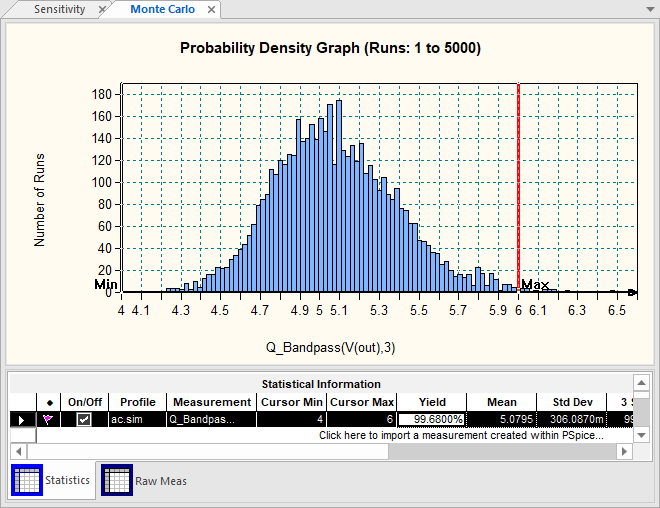
Only one over 200 circuit is now out of specification with Q=6.1. That's much better, we can sell 99.5% of the production!

To get an idea of the actual distribution law of the Q factor, you'll have to generate more runs. The below result reveals a Gaussian distribution obtained over 5000 runs. It is often the case (Gaussian), but not always depending on circuit non-linearities. It took 00:33:41 to get the simulation result, with a yield that is not very different from the one obtained with only 200 runs and about 00:01:30 simulation time.